
Sometimes you just want to deploy an ML model without using fancy tools.
When you had your first machine learning lessons, probably one of your first thoughts “ok now I trained my model, how can I use it in a real application?”.
If you work with ML-related cloud tools (AWS SageMaker, GC vertex AI, Azure Machine Learning, etc.), you know how easy it can be to configure and deploy a machine learning model so it can be in inference mode, starting to make predictions with real data. However, this can not be the case due to different reasons, here and example:
- You work in a company where paying for a ML cloud-based service is not worth it. probably because the proyect is too small, a PoC, or it’s not planned to last alive for long time
- Your infrastructure is on-premise
- The deployed model is hosted in an intranet, so there’s no internet connection
- All the previous points + you’re budged limited
Besides all the previous points, it’s a good idea to know how services work behind scenes, especially if this big world is new to you.
This blog post, includes different areas for a machine learning solution, from using the dataset to train the model until you have an endpoint in your local computer. Putting this endpoint in a production environment is up to you since it will depend on your infrastructure.
For this tutorial, we’ll create an endpoint that will predict the type of iris plant based on the sepal and petal measures (yes, the classic iris problem with the classic iris dataset). You’ll need Python for sure. I’ll be using scikit-learn as the machine learning library and Flask as the webserver. You can use the libraries of your choice (TensorFlow, PyTorch, Django…) since this post focuses on how to deploy the trained model.
You can find the source code and instructions on how to set up this project in my Github repository.
Creating the ML model
As mentioned before, our dataset contains data of 150 iris plants. The columns are:
- sepal_length, in cm
- sepal_width, in cm
- petal_length, in cm
- petal_width, in cm
- class, which can be one of these three:
- Iris-setosa
- Iris-versicolour
- Iris-virginica
The first 4 columns will be our independent variables and the class column our dependent variable:
Here comes the important part. As you know, data has some problems if we want to start training and predicting with it just as it is:
- If you don’t scale numeric values, some features can have more weight than others, for example salary vs age, even if in some cases age could be more important.
- Categorical variables need to be converted into dummy variables and avoid the dummy variable trap.
These and other transformations on the data are easy to perform, but they need to be consistent, for example, to remember the dummy variables column order, or knowing which dummy variable was omitted. To solve this problem, you’ll need to preserve all the transformers you use during your training, and, in the same way, you’ll need to preserve the model itself.
In this sample project, we are using only one scaler:
But for any extra transformer, keep an individual object. This means, that, for example, if you have two columns with categorical values, you’re going to need two OneHotEncoder objects, one per column.
We need to do the same with our model, in this case, our classifier:
Once you have trained, validated, and tested the model, and you are happy with it, now it’s the moment of the truth, to serialize the model and the scaler. To do that, we’ll use the dump function from the joblib module:
Creating the endpoint
Now that we’ve trained and saved our model, let’s create an API endpoint to consume it sending the plant data, and return the prediction in a JSON format.
This endpoint will be created using Flask. If you have never used it before, find more details on how to configure it in the project repository or the official Flask documentation.
The important things to remark here:
- In line 2, we are loading the
loadfunction from thejoblibmodule. This function is how we’ll deserialize the scaler and the model. - In line19, we create a two dimmensions array named
plant. It contains the 4 necessary independent variables we need to predict to which iris plant these features belong. - In line 21, we are loading the standard scaler. If you have serialized more scalers, one hot encoders or any other object, this is the time to load them.
- In line 22 we do the same, we load the trained model.
- In line 24 we scale the feature values.
- In line 25 the model predicts which is in the array, it returns an array with all the predictions (in this case only one)
- In line 27, we return the predicted class.
Testing the solution
Now that we have everything set, it’s time to test everything all together.
In the repository, the endpoint folder includes a file called endpoint_tester.py. It’s a very basic file that makes a call to the local endpoint.
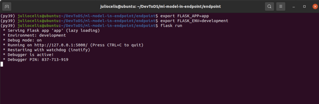
First, we need to run the Flask application. Open a terminal/command line, navigate to the endpoint folder to configure and run Flask:
For Windows:
> set FLASK_APP=app
> set FLASK_ENV=development
For macOS and Linux:
$ export FLASK_APP=app
$ export FLASK_ENV=development
After that, in the terminal/command line run the next command:
flask run
Keep the console open, it will show a similar message to this:
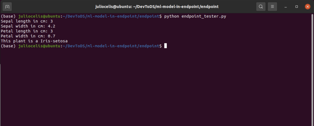
In another terminal/command line, navigate as well to the endpoint folder and run the next command:
python endpoint_tester.py
This command will show you a prompt asking you for the plant properties and after you enter the four, it will call the endpoint and display the plant type:
Conclusion
Putting a trained model in inference mode is not complicated when you need to do it manually. Nowadays, this approach is not the most popular, but it helps a lot to understand the full lifecycle since this part is something not taught in ML courses.